As Featured in PE&RS: Cutting-edge LiDAR Quality Control Methods Revealed in February 2024 Issue
When it comes to geospatial data, ensuring the accuracy and precision of LiDAR point clouds is paramount for creating reliable map products. In the February 2024 issue of Photogrammetric Engineering & Remote Sensing (PE&RS), a team from our sister company GeoCue, including Martin Flood, Dr. Nicolas Seube, and Darrick Wagg, authored an article that concentrated on LiDAR Point Cloud Quality Control: Automating Accuracy and Precision Testing.
With a focus on automating accuracy and precision testing, this article explains the evolving landscape of quality assurance in the realm of LiDAR data processing. As LiDAR technology continues to advance and find applications in diverse sectors, from large-scale surveying to drone-based data collection, the need for efficient quality control mechanisms becomes increasingly apparent. The article is now available in the February edition of the PE&RS Journal, or below.
Lidar Point Cloud Quality Control: Automating Accuracy and Precision Testing
The creation of map products from lidar point clouds requires rigorous quality control procedures. Review processes include manual inspection (“eyes on”) by a qualified technician in an interactive point cloud editing environment and increasingly automated quality checking tools to measure accuracy, precision, and other quality metrics. Increasing the efficiency of this review process is an important research area for lidar data producers and data users. Smaller lidar surveys, such as those collected by drones, require the same quality review and assessment tools for measuring accuracy and precision as larger scale surveys, so they can benefit from more automation as well.
In this article, we report on improved methods to automatically assess the accuracy and precision of lidar point clouds. We reference the ASPRS Positional Accuracy Standards for Digital Geospatial Data (2nd Edition) (the ‘ASPRS Standard’ or the ‘Standard’) throughout as the authoritative reference for lidar data quality assessment and reporting for map products. First, we will discuss the automatic detection of 3D lidar targets (“Accuracy Stars”) in point cloud data to measure vertical and horizontal accuracy and derive translation/rotation corrections for the data. In the second part of the article, we discuss our use of computational geometry to measure and report precision over large project areas using Principal Component Analysis (PCA). Combined, these two techniques allow for more automated quality checking of lidar point cloud accuracy and precision, reducing the need for manual interaction and scaling efficiently over large (or small) project areas.
Accuracy
Lidar accuracy assessment is typically done via classical methods inherited from photogrammetry. Vertical accuracy checking against the lidar surface at a known checkpoint (survey nail) is the most common approach in use today. Surface modelling of the lidar data is done using accepted Triangular Irregular Network (TIN) or Inverse Distance Weighted (IDW) methods. The orthogonal distance between the checkpoint and the lidar surface gives the vertical error. Using a collection of such checkpoints provides the statistical Root Mean Square Error (RMSE) in the vertical for the surface, assuming the checkpoints are well-distributed across the area. A minimum of 30 checkpoints are required by ASPRS for “Tested to Meet …” accuracy reporting. Many drone lidar projects will have less than 30 checkpoints and will be reported as “Produced to Meet …”. Specific wording for each of these cases is outlined in the Standard, Section 7.15.
The fit of a product (the lidar surface) to known checkpoints is the First Component of Positional Error. It is what has been traditionally reported as the “accuracy” of lidar data by vendors and data producers. With the increasing accuracy of lidar sensors, the ASPRS Standard now acknowledges the inherent error in the position of the checkpoints themselves is becoming significant and must also be considered when reporting the accuracy achieved. The uncertainty (error) in the checkpoint position, typically reported by the surveyor collecting the checkpoints, needs to be included in the final stated product accuracy. The statistical RMSE value of the checkpoint positions is referred to as the Second Component of Positional Error. Product accuracy is the Root Sum of Squares Error (RSSE) of the two components. See Section 7.11 in the Standard for details. Practically, this means for lidar datasets the reported accuracy cannot be better than the checkpoint accuracy and typically will be slightly higher than the surface-to-checkpoint value measured by traditional point-to-TIN methods. Users should not assume this checkpoint error contribution is negligible when assessing a lidar system’s achievable accuracy for a derived mapping product.
Horizontal positional accuracy is reported like vertical accuracy, with both First and Second component errors contributing to the final horizontal accuracy. Reporting is typically done as the radial or planimetric (XY) accuracy achieved rather than as individual single-axis errors. Traditionally, lidar datasets have used identifiable visible targets in the point cloud for horizontal error measurement. These can be specific targets deployed during the survey flights, like photogrammetric panels, or targets of opportunity that have been surveyed, such as building corners, manhole covers, road markings etc. The planimetric (XY) position of such targets in the point cloud is collected manually in post-processing, but this is labor-intensive and prone to interpretation error in the manual capture. Automating both the vertical and horizontal accuracy checking using detection algorithms to identify and locate the targets reduces the labor required, is less prone to user error, eliminates errors of interpretation in target location, and allows for a more rigorous calculation of offsets and corrections to be applied to the point cloud.
Our algorithmic approach to target detection relies on using monumented Ground Control Targets (GCTs) that can be “seen” within the point cloud. Such targets can be 2-dimensional (XY) such as checkerboard or concentric targets on the ground or they can be 3-dimensional (XYZ) objects such as spheres or discs configured in a well-defined pattern and mounted above the ground. Color contrast, such as alternating black and white segments, or high-reflectivity paint is used to enhance the detectability in the point cloud.
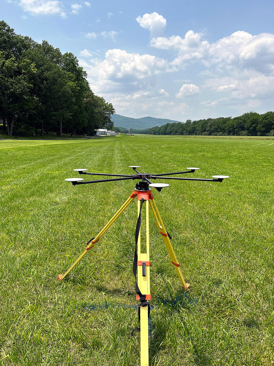
A recent field test was performed with our partners at Earl Dudley, LLC to assess the accuracy of a TrueView 680 (Riegl VUX-based design) drone lidar survey of a highway intersection. A single Accuracy Star (AS) was set up over a known survey point. Two passes of the TrueView 680 were flown and the data post-processed in LP360 to a georeferenced and strip-matched point cloud. The target detection algorithm identified the AS in the point cloud with a high degree of confidence due to the point density and open sky above the target. The XYZ offsets measured using the AS were used to automatically apply a correction to the point cloud. The adjusted point cloud was then compared to 21 photogrammetric panel points surveyed by total station and digital level. The resulting RMSE(z) was 0.33 cm (0.011 feet). The surveyed positional accuracy RMSE(z) (First Component) of the AS was 0.5 cm (0.016 feet) (Second Component) for a final total RMSE(z) for the lidar surface of 0.57 cm (0.019 feet).
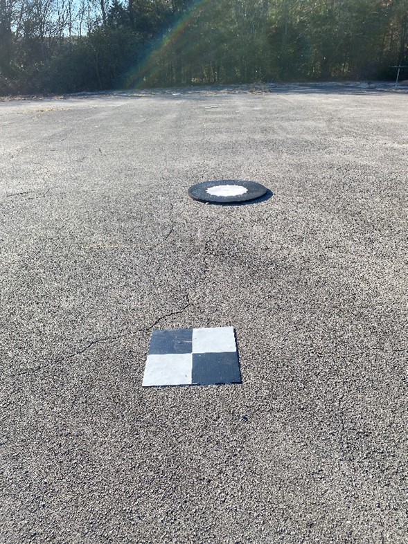
The use of 3D targets such as the Accuracy Star is not always required on a project. By extending the target detection algorithm to work with more traditional checkerboard targets and concentric circle targets, examples of which are shown in Fig 2, the same automated tools can be applied. This allows for XYZ offsets and corrections to be automatically extracted from the 2D targets, but not a full 6-degree solution with rotation. This is a practical intermediate use case for most surveyors; a more rigorous solution than traditional survey nails (Z assessment only) but requiring less set-up and hardware than a full set of 3D targets.
Precision
For lidar datasets, precision is commonly interpreted as the repeatability of the point data without regard to survey control or network accuracy. Practically it is a measure of the noise or “fuzziness” of the point cloud on a hard surface such as a road or roof. Many factors contribute to the precision of a given lidar sensor; laser shot noise, sensor stability, consistency of the position solution, rigidness of the calibration and boresight to name a few. The ASPRS Standard defines two measures of precision of interest to lidar data users; within-swath (intraswath or smooth surface precision) which applies to data from a single pass of the instrument, and swath-to-swath, (or interswath precision) which applies to data in the overlap area of two or more passes.
Historically, assessment of precision has been done by determining the noise level of the point cloud on test surfaces (e.g., impervious hard surfaces). Recommended test methods include creating an elevation difference raster and computing a RMSE between min/max elevations (smooth surface) or between flight lines (interswath dZ) in each cell or performing a planar fit to the test surface and reporting the standard deviation of the fit. These values are then compared to the precision tolerances allowed for a given vertical accuracy class (see Table 7.2 in the Standard). The general guideline is that the smooth surface precision (within swath) should be no greater than 0.6x the vertical accuracy class required for the derived map product. Restrictions on the allowable swath-to-swath value for a given Quality Level (QL) level are also documented.
The test methods for smooth surface precision (within swath) are limited to spot-checking areas and often are labor-intensive, for example to identify suitable test plots for the analysis. They do not scale well to large projects. The Standard does not state a specific number of test points for precision assessment but does recommend testing precision “to the greatest extent possible” (see Section C.10). A more automated, comprehensive test of the precision achieved over the entire project area is desirable. To develop such methods, we have been investigating applying computational geometry techniques based on a Principal Component Analysis (PCA) of the point cloud across the entire dataset. We want a rigorous, automated way to measure precision (noise) on smooth surfaces across both large and small data sets and present both qualitative and quantitative results back to the user. We want the measurements to be unbiased with respect to local slope and curvature of the terrain. We also assume no apriori information on the location of these smooth surfaces is available.
The approach we have been developing involves calculating the standard deviation along the surface normal (SDASN) for a given cell size across the entire project area. To accomplish this, we apply a Principal Component Analysis (PCA) to measure the local linearity, planarity, and sphericity of the neighborhood. While this analysis could be run for each individual point using a spherical neighborhood in 3D space, for computational efficiency we use a raster approach with a 2D grid and apply the PCA analysis to each cell in the grid. This gives us linearity, planarity, and sphericity, along with the standard deviation along the surface normal (SDASN) for each cell. This also gives us an estimate of local curvature for each cell by calculating the corresponding surface variation from the PCA parameters.
The measurement of smooth surface (intraswath) precision follows directly from the above analysis. The algorithm identifies cells with a high level of planarity, a low level of sphericity, and an absence of local curvature. Cells that meet these criteria are taken as planar (smooth) but are not necessarily horizontal. They have a SDASN that is an unbiased (by local slope and curvature) measure of precision of the point cloud in that cell. Unlike a basic dZ check that measures min/max elevation differences in a cell, SDASN quantifies the deviation of the points perpendicular to the planar fit to the local surface. We rasterize the entire grid to colorize the cells for qualitative analysis (like the popular “dZ” rasters used for overlap assessment) and extract the numerical values for a quantitative statistical analysis. The analysis can be restricted to only planar cells within a single flight line (intraswath) or planar cells with multiple flight lines (interswath), depending on the use case. The user is presented with a greyscale or colorized raster that highlights only those planar surfaces that exceed the specified value (for Pass/Fail testing) or based on a color ramp of user-defined bands. Quantitative measurements of the precision can also be extracted during the analysis. This approach allows for rapid assessment of lidar data precision in an automated and comprehensive method across the entire project area, automatically identifying those surfaces appropriate for precision testing.
Several examples of SDASN analysis are presented below from field tests conducted using a TrueView drone lidar system for small site testing and using publicly available 3DEP lidar data for broad area tests. All analysis was performed in the LP360 software suite using SDASN tools in development for future release.
The 3DEP project chosen for testing was from Utah; UT_StrawberryRiver_2019. This area is forested, with steep elevations and limited road access. The test data comprised 152 LAS files covering ~100 sq. mi. with 100 GB of QL1 data. The data was previously ground classified, allowing for the SDASN analysis to be performed against the ground surface. An example of the resulting raster product is shown in Fig. 3. This is a 5 sq. mile area rasterized with 2 m pixels showing the relative SDASN (noise) values from Low (Black) to High (White) for the ground class. Terrain structure is revealed along with areas of high relative noise in the point cloud that indicate potential problem areas.

The choice of cell size is an interesting one and we are continuing to investigate this parameter. For a rigorous PCA result, we want 10+ points per cell. The confidence level of the results drops off as we move to less dense data. Practically, we think this means we will need at least four points per sq. m to achieve minimum acceptable results. Our approach works well for QL1 or better data (or on dense drone lidar datasets) but will be less reliable for sparser QL2 data. We are investigating ways to increase the reliability with less dense data (beyond just increasing the cell size) to get more reliable results with QL2 data sets.
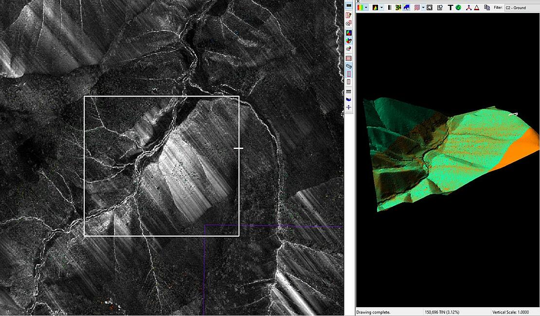
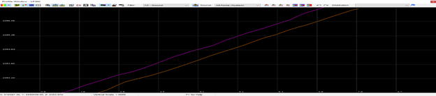
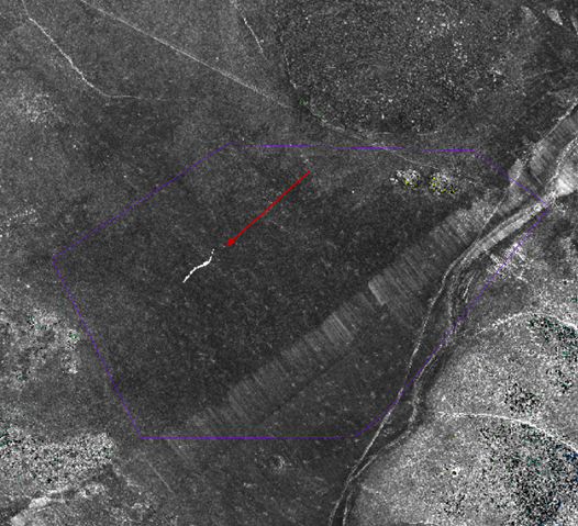
Investigating the potential problem areas, Fig. 4 and Fig. 5 show a section of high noise on the side of a steep slope that, upon closer investigation, reveals a dynamic drift between flight lines that increases to a maximum of 45 cm before returning to within tolerance further along the flight line. Due to the remote location and lack of flat, open surfaces, such a dynamic error would not have been identified by the traditional sample plot testing for swath-to-swath precision.
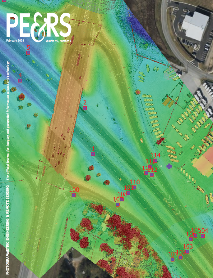
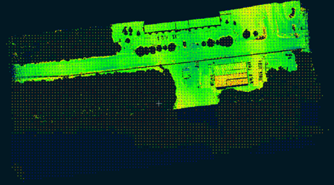
Investigating small sites surveys, Fig 6. shows a SDASN raster for a drone lidar (TrueView 535) flight used to assess sensor calibration and boresight. In this use case the PCA analysis has been limited to only 0.5 m planar cells. The colorization is from Low/Green (< 2 cm) to High/Red (> 8 cm) and shows the smooth surface precision (intraswath) on flat surfaces (the road, parking lots, and building roofs). The point data is unclassified. RMSE of the precision was 1.2 cm.
Finally, as a secondary use for SDASN, we have been examining using the rasters to assist in the QC of the lidar ground surface. Misclassifications of the ground points often characterize as deviations from a smooth surface and an SDASN analysis can make these areas visually “pop” for the reviewer in the QC raster. We are investigating how to optimize this use case further and extend it to other features such as buildings. Fig 7. shows an example of a bust in the ground class easily identified in the SDASN QC raster.
In conclusion we have observed significant improvements in the efficiency and the reliability of quality checks performed on lidar point clouds by using automated 3D target detection for accuracy assessment and data correction and Standard Deviation Along Surface Normal (SDASN) analysis for precision assessment over an entire project area. These techniques apply equally well to both large and small project sites.
If you have more questions about LiDAR Point Cloud Quality Control, schedule a meeting to speak with one of our LiDAR Experts today.